Parameters initialization impacts

About

This page contains notes from Karpathy's YouTube lecture Building makemore Part 3: Activations & Gradients, BatchNorm . I downloaded the video and generated captions using generate_captions.py. wherever "I" is seen, it refers Karpathy.

1. Initial setting

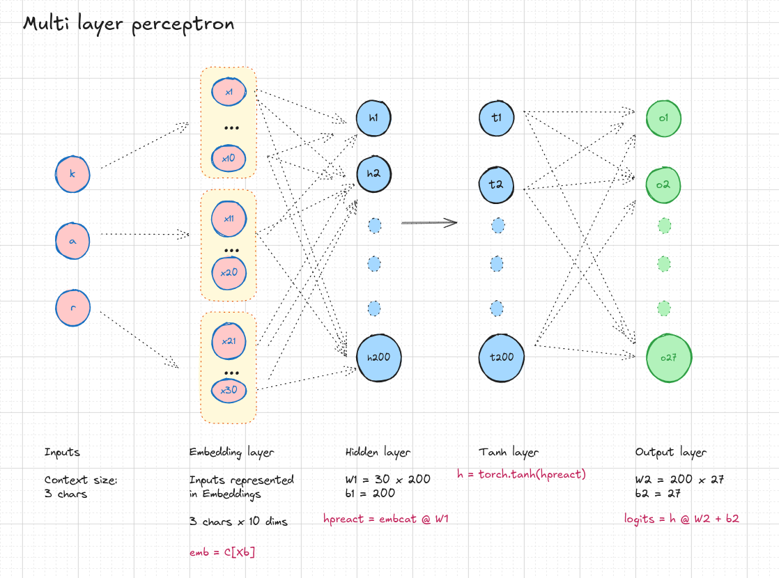
# MLP revisited  
n_embd = 10  # the dimensionality of the character embedding vectors  
n_hidden = 200  # the number of neurons in the hidden layer of the MLP  
  
g = torch.Generator().manual_seed(2147483647)  # for reproducibility  
C = torch.randn((vocab_size, n_embd), generator=g)  
W1 = torch.randn((n_embd * block_size, n_hidden), generator=g)  
b1 = torch.randn(n_hidden, generator=g)  
W2 = torch.randn((n_hidden, vocab_size), generator=g)  
b2 = torch.randn(vocab_size, generator=g)

# forward pass  
emb = C[Xb]  # embed the characters into vectors  
embcat = emb.view(emb.shape[0], -1)  # concatenate the vectors  
  
# Linear layer  
hpreact = embcat @ W1  #+ b1 # hidden layer pre-activation  
  
# Non-linearity  
h = torch.tanh(hpreact)  # hidden layer  
logits = h @ W2 + b2  # output layer  
loss = F.cross_entropy(logits, Yb)  # loss function

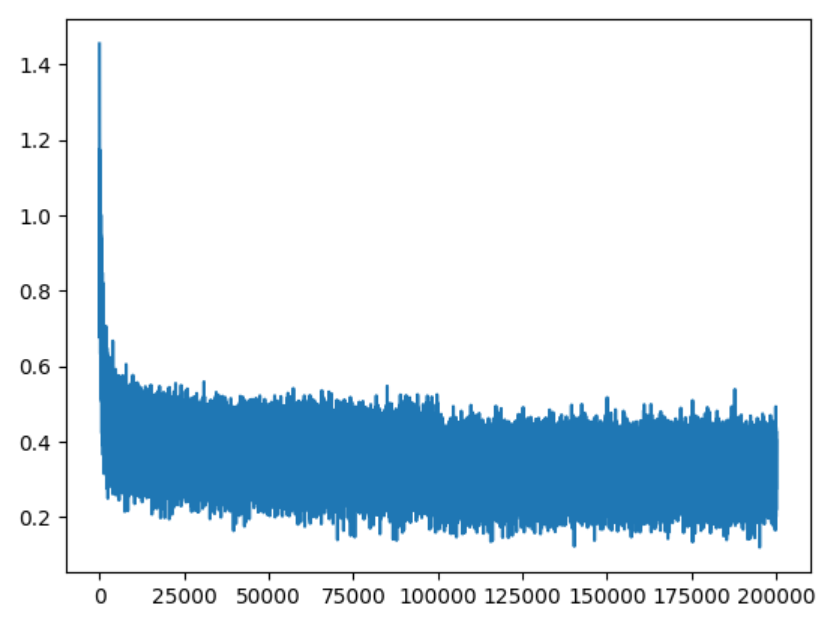
training loss

      0/ 200000: 28.4938
  10000/ 200000: 2.7052
  20000/ 200000: 2.5689
  30000/ 200000: 2.7037
  40000/ 200000: 2.0714

---

2. What's wrong with the model?

I can tell that our network is very improperly configured at initialization, and there's multiple things wrong with it, but let's just start with the first one - Look here on the 0th iteration, the very first iteration, we are recording a loss of ~ 27, and this rapidly comes down to roughly one or two or so. so I can tell that the initialization is all messed up because this is way too high. In training of neural nets, it is almost always the case that you will have a rough idea for what loss to expect at initialization, and that just depends on the loss function and the problem set up. In this case, I do not expect 27. I expect a much lower number, and we can calculate it together.

Basically, at initialization, what we'd like is that there's 27 characters that could come next for any one training example. At initialization, we have no reason to believe any characters to be much more likely than others. and so we'd expect that the probability distribution that comes out initially is a uniform distribution, assigning about equal probability to all the 27 characters.

# Each of the 27 chars have equal probability.
# Expected initial loss (Negative Log Likelihood)
-torch.tensor([1 / 27]).log()

tensor([3.2958])

what's happening right now is that, at initialization, the neural net is creating probability distributions that are all messed up. Some characters are very confident and some characters are very not confident. And then basically what's happening is that the network is very confidently wrong and that's what makes it record very high loss.

---

3. Changes to initialization

1. Weights Initialization

We don't want logits to be any arbitrary positive or negative number, we just wanted to be all zeros and record the loss that we expect at initialization.

# MLP revisited
n_embd = 10  # the dimensionality of the character embedding vectors
n_hidden = 200  # the number of neurons in the hidden layer of the MLP

g = torch.Generator().manual_seed(2147483647)  # for reproducibility
C = torch.randn((vocab_size, n_embd), generator=g)
W1 = torch.randn((n_embd * block_size, n_hidden), generator=g)
b1 = torch.randn(n_hidden, generator=g)
W2 = torch.randn((n_hidden, vocab_size), generator=g) * 0.01
b2 = torch.randn(vocab_size, generator=g) * 0

parameters = [C, W1, b1, W2, b2]
print(sum(p.nelement() for p in parameters))  # number of parameters in total

for p in parameters:
    p.requires_grad = True

Changes done:

• W2 is multiplied by 0.01
• b2 is multiplied by 0 to make the logits near 0.

With this change, the initial loss is ~ 3.32 compared to ~27 earlier.

      0/ 200000: 3.3277
  10000/ 200000: 2.2796
  20000/ 200000: 2.4154
  30000/ 200000: 2.6209
  40000/ 200000: 1.9621

2. Tanh activations

• The problem now is with the values of h, the activations of the hidden states.
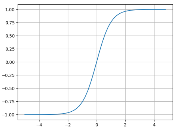
• Now, if we just visualize this vector, h you see how many of the elements are 1 or -1
• Recall that tanh is a squashing function. It takes arbitrary numbers and it squashes them into a range of -1 and 1, and it does so smoothly.

import numpy as np
import matplotlib.pyplot as plt
%matplotlib inline

plt.plot(np.arange(-5, 5, 0.2), np.tanh(np.arange(-5, 5, 0.2)))
plt.grid()

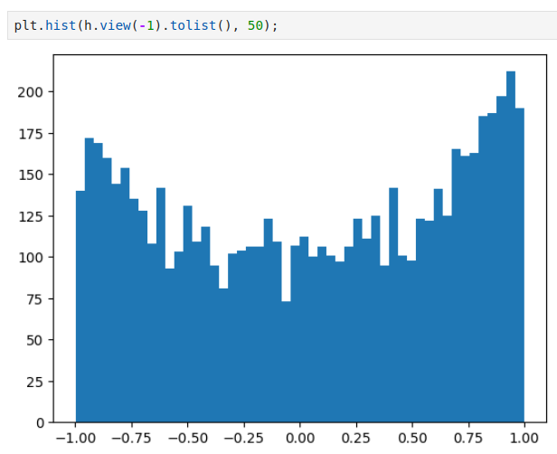
# View the distribution in tensor h
plt.hist(h.view(-1).tolist(), 50);

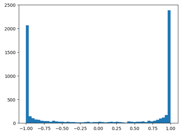
• we see that most the values by far take on value of -1 and 1, so the tanh is very very active.

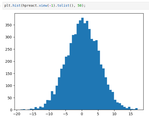
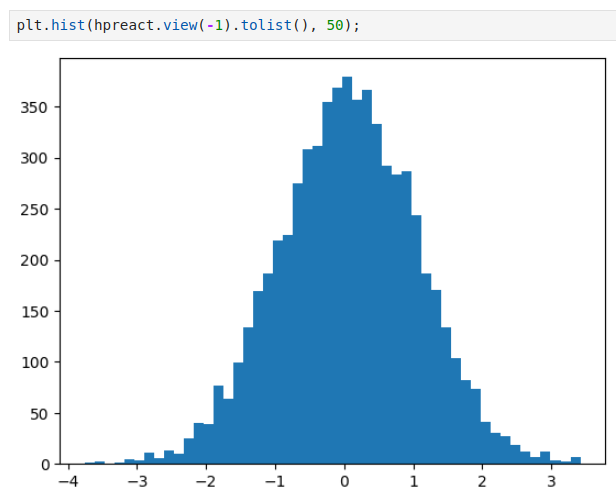
we can look at the pre-activations that feed into the tanh and we can see that the distribution of the pre-activations are, is very, very broad.
These take numbers between -15 and 15, and that's why in a tanh, everything is being squashed and capped to be in the range of negative -1 and 1, and lots of numbers here take on very extreme values.

What happens when Tanh takes high values?

We have to keep in mind that during back-propagation, we are doing backward pass, starting at the loss, and flowing through the network backwards In particular, we're going to back-propagate through this tanh

# Gradient of tanh  
self.grad += (1 - t ** 2) * out.grad  
  
# where "t" is the value of tanh(activation)

• When t = -1 or 1, there is no change in gradient.
• This means, During backward pass, the gradient is killed and the weights are not updated.
• No matter what out grad is, we are killing the gradient, and we're stopping effectively the back propagation through this tanh unit.

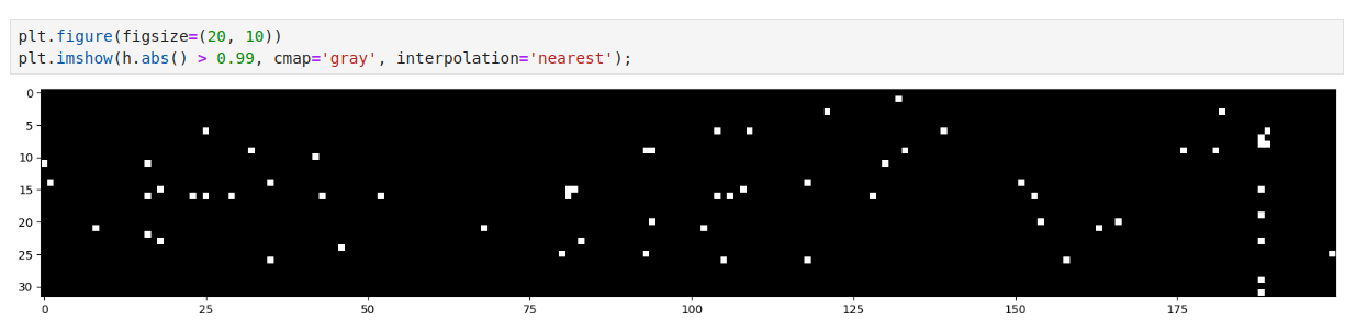
# For a batch, plot the hidden state values (h)
#   h > 0.99: For these values tanh will be 1 (These are shown as white color)
plt.figure(figsize=(20, 10))
plt.imshow(h.abs() > 0.99, cmap='gray', interpolation='nearest');

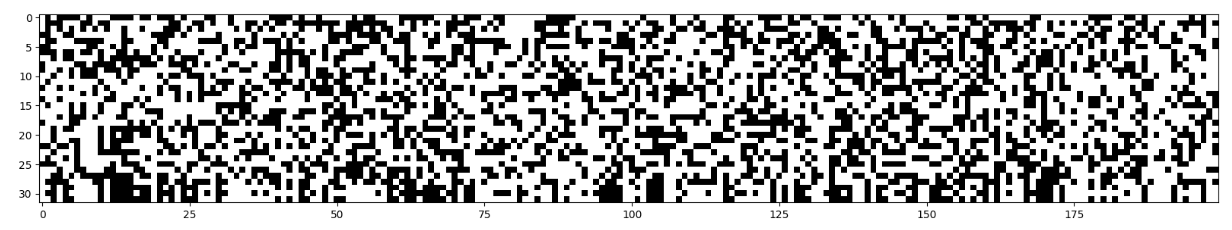
• Now, we would be in trouble if, for any one of these 200 neurons, if it was the case that the entire column is white because in that case we have what's called a dead neuron.

Update weights W1, b1

# MLP revisited  
n_embd = 10  # the dimensionality of the character embedding vectors  
n_hidden = 200  # the number of neurons in the hidden layer of the MLP  
  
g = torch.Generator().manual_seed(2147483647)  # for reproducibility  
C = torch.randn((vocab_size, n_embd), generator=g)  
W1 = torch.randn((n_embd * block_size, n_hidden), generator=g) * 0.2  
b1 = torch.randn(n_hidden, generator=g) * 0.02  
W2 = torch.randn((n_hidden, vocab_size), generator=g) * 0.01  
b2 = torch.randn(vocab_size, generator=g) * 0

Activation (h)	Preactivations (hpreact)
Now, the hidden state values are between -1 and 1.

Training loss now is:

      0/ 200000: 3.3134
  10000/ 200000: 2.1660
  20000/ 200000: 2.3240
  30000/ 200000: 2.3918
  40000/ 200000: 1.9870

• And the reason this is happening, of course, is because our initialization is better, and so we're spending more time doing productive training instead of not very productive training because our gradients are set to zero, and we have to learn very simple things like the overconfidence of the softmax in the beginning, and we're spending cycles just like squashing down the weight matrix
• So this is illustrating basically initialization and its impacts on performance just by being aware of the internals of these neural nets and their actuations and their gradients
• Now, we're working with a very small network - This is just one layer multilayer perception. So because the network is so shallow, the optimization problem is actually quite easy and very forgiving. So even though our initialization was terrible, the network still learned eventually it just got a bit worse result.
• This is not the case in general, though. Once we actually start working with much deeper networks that have, say, 50 layers, things can get much more complicated, and these problems stack up. And so you can actually get into a place where the network is basically not training at all if your initialization is bad enough And the deeper your network is and the more complex it is, the less forgiving it is to some of these errors. and so something to we definitely be aware of and something to scrutinize, something to plot, and something to be careful with.

---

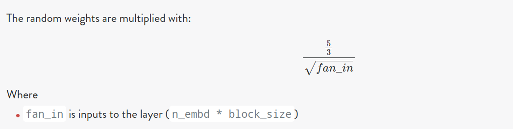
4. Determining scaling factor

Okay, so that's great that that worked for us, but what we have here now is all these match of numbers, like 0.2, like where do I come up with this? And how am I supposed to set these if I have a large neural net with lots and lots of layers? And so obviously no one does this by hand. There's actually some relatively principled ways of setting these scales that I would like to introduce to you now.

Kaiming Initialization

• Delving Deep into Rectifiers: Surpassing Human-Level Performance on ImageNet Classification
• torch.nn.init

W1 = torch.randn((n_embd * block_size, n_hidden), generator=g) * ((5/3) / ((n_embd * block_size) ** 0.5))

This is implemented in PyTorch as kaiming_uniform

---

5. Improvements

There are a number of modern innovations that have made everything significantly more stable and more well-behaved, and it's become less important to initialise these networks exactly right. And some of those modern innovations, for example, are:

• Residual connections
• The use of a number of normalization layers, like, for example, batch normalization, layer normalization, group normalization
• Better optimizers, like RMS prop, Adam And so all of these modern innovations make it less important for you to precisely calibrate the initialization of the neural net.